Boundary Conditions
Now that we have the global stiffness matrix \(\boldsymbol{K}\) we can write out the system of linear equations in the following way:
where \(\boldsymbol{u}\) denotes the displacement and \(\boldsymbol{f}\) the forces. Just to remind you, the structure of \(\boldsymbol{u}\) and \(\boldsymbol{f}\) is as follows:
where \(u_{ix}\) and \(u_{iy}\) denote the \(x\) and \(y\) displacement of the \(i\)th node, respectively. \(f_{ix}\) and \(f_{iy}\) denote the force acting on the \(i\)th node in \(x\) and \(y\) direction, respectively.
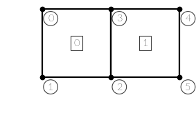
Consider a system defined via
from fem.node import Node
from fem.element import Element
from fem.system import System

nodes = [Node(0, 1),
         Node(0, 0),
         Node(1, 0),
         Node(1, 1),
         Node(2, 1),
         Node(2, 0)]

elements = [Element(nodes[:4], 3e7, 0.3),
            Element(nodes[-1:1:-1], 3e7, 0.3)]

system = System(elements)
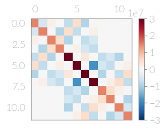
Now you can take a look at the global stiffness matrix:
What is missing are \(\boldsymbol{u}\) and \(\boldsymbol{f}\). As \(\boldsymbol{u}\) is the solution only \(\boldsymbol{f}\) – the loading – has to be defined. And as always there is a special name, even for this kind of boundary condition: Neumann boundary conditions.
Neumann Boundary Conditions
When a loading is prescribed it is a so-called Neumann boundary condition. If the loading is prescribed directly at the nodes in form of a point force it is sufficient to just enter the value in the force vector \(\boldsymbol{f}\). Assume a force of magnitude 10 acts on node 5 in \(x\) direction and 0 at all other degrees of freedom. Hence \(\boldsymbol{f}\) looks like this:
In the code this should be handled by an attribute of the system with the name
neumann_bc. This attribute should be a dict whose keys are the
indices of the degrees of freedom and whose values are the forces that are
prescribed. This attribute shall then be used by the following method that you
shall implement:
-
System.assemble_force_vector()¶ Return the right hand side of the system taking Neumann boundary conditions into account.
Returns: The global right hand side of the system. Return type: numpy.ndarray
With this you are able to prescribe forces on nodes. This is, however, not sufficient to solve the system, even though a solver routine might not give you an error or even a warning a quick look at the result should tell you that something is really, really fishy:
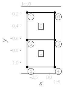
Note how the size of the body suddenly is of the size \(10^9\). So by only applying one force at a single node in your body you blew up the body tremendously? The error is that by only applying Neumann boundary conditions the system has an infinite amount of solutions. The body could be moving in \(x\) direction, in \(y\) direction,it could be turning in the \(xy\) plane, or a combination of those. These are called the rigid body motions. To remedy this you have to “pin” the body somewhere – that is you have to prescribe the displacements of certain nodes so that your system has a unique solution. And like prescribing forces prescribing displacements has a name: Dirichlet boundary conditions.
Dirichlet Boundary Conditions
Prescribing displacements directly is a bit more involved than simply prescribing point loads. Suppose you wanted to pin node 0 in \(x\) and \(y\) direction and node 3 in \(x\) direction to eliminate the three rigid body modes (three constraints for three rigid body modes). They correspond to the degrees of freedom 0, 1 and 6. In order to constrain them the displacement vector \(\boldsymbol{u}\) will be split in two parts – the prescribed part \(\boldsymbol{u}_{\Gamma}\) and the unknown part \(\hat{\boldsymbol{u}}\). It follows
which after reordering results in
Subsequently the global stiffness matrix on the left hand side has to be reduced by setting the columns and rows of the degrees of freedoms that are prescribed to zero, except for the common element which is set to one.
where
At this point you may implement the
get_reduced_system() method according to the
specifications given. Use the other methods you already implemented inside of
this method to retrieve the system without applied boundary conditions.
-
System.get_reduced_system()¶ Return the reduced global stiffness matrix and right hand side taking all boundary conditions into account.
Returns: - K_reduced (numpy.ndarray) – The reduced global stiffness matrix
- rhs (numpy.ndarray) – The reduced global right hand side
Now you can calculate the right hand side and get your solution using a solver
for systems of linear equations, for example a direct solver, a conjugate
gradient solver or the solver that comes with NumPy –
numpy.linalg.solve(). Use this in a solve()
method that is specified as follows:
-
System.solve()¶ Return the solution vector of the system.
Returns: Solution vector of the system. Return type: numpy.ndarray