Post-Processing¶

Strain¶

Remember that the strain \(\boldsymbol{\varepsilon}\) is defined as the symmetric gradient of the displacements \(\boldsymbol{u}\):

\[\boldsymbol{\varepsilon} = \boldsymbol{\nabla}_{\mathrm{sym}} \boldsymbol{u}\]

or in index notation

\[\varepsilon_{ij} = \frac{1}{2} \bigl(u_{i, j} + u_{j, i}\bigr)\]

In our finite element implementation we used the Voigt notation for the strains and stresses, hence this formula has to be adapted according to this notation. This is will be “automatically” taken care of when we use the shape function gradient matrix \(\boldsymbol{B}\). When you are using the finite element method you typically compute the strains on the element level using the symmetric shape function gradients:

\[\boldsymbol{\varepsilon}^{e}(\xi, \eta) = \boldsymbol{B}^{e}(\xi, \eta) \boldsymbol{u}^{e}\]

Implement a method in the Element class that computes the strain vector at the position \(xi\), \(eta\) according to the following specifications:

Element.strain(xi, eta, u)¶

Return the strain vector of the element subject to displacements u at the reference space position (xi, eta).

Parameters:	xi (float) – Reference space coordinate at which the strain should be computed. eta (float) – Reference space coordinate at which the strain should be computed. u (numpy.ndarray) – Global displacement vector that results from `solve()`.
Returns:	The strain vector of the element subject to displacements u at position (xi, eta) given as \(\begin{bmatrix} \varepsilon_{xx} & \varepsilon_{yy} & \varepsilon_{xy} \end{bmatrix}^{\mathrm{T}}\).
Return type:	numpy.ndarray

Stress¶

Using the strains computing the stresses is straightforward via the popular Hooke’s law

\[\boldsymbol{\sigma} = \boldsymbol{C} \boldsymbol{\varepsilon}\]

which in terms of a finite element is usually handled via

\[\boldsymbol{\sigma}^{e}(\xi, \eta) = \boldsymbol{C}^{e} \boldsymbol{\varepsilon}^{e}(\xi, \eta)\]

Implement a method in the Element class that computes the stress vector at the position \(xi\), \(eta\) according to the following specifications:

Element.stress(xi, eta, u)¶

Return the stress vector of the element subject to displacements u at the reference space position (xi, eta).

Parameters:	xi (float) – Reference space coordinate at which the stress should be computed. eta (float) – Reference space coordinate at which the stress should be computed. u (numpy.ndarray) – Global displacement vector that results from `solve()`.
Returns:	The stress vector of the element subject to displacements u at position (xi, eta) given as \(\begin{bmatrix} \sigma_{xx} & \sigma_{yy} & \sigma_{xy} \end{bmatrix}^{\mathrm{T}}\).
Return type:	numpy.ndarray

Plotting Fields¶

Now that you have your finite element code up and running it is time to see the results of your hard work. For this a function is provided:

plot_mesh(ax, elements, u=None, u_amp=1, field=None, field_label=None, field_resolution=4, padding=0.1, show_axes=True, verbose=True)¶

Plot a finite element mesh and – if given – its solution and fields.

Parameters:

ax (matplotlib.axes.Axes) – The axes which the mesh should be plotted in.
elements (list[fem.element.Element]) – List of elements that make up the mesh that should be plotted.
u (numpy.ndarray) – Solution of the FEM system returned by solve().
u_amp (float) – Amplification of the displacements u.
field (function) – Function with the interface f(element, xi, eta, u) where element is an Element, xi and eta are reference coordinates and u is the solution of the FEM system returned by solve().
field_label (str) – Name of the field that should be plotted.
field_resolution (int) – Amount of partitions the field interpolation should use.
padding (float) – The padding of the axis figure.
show_axes (bool) – Whether to show the axes or not.
verbose (bool) – Whether to show the element and node numbers or not.

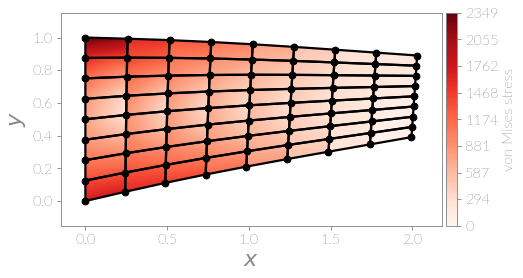
Using this you can plot the results:

#!/usr/bin/env python
# -*- coding: utf-8 -*-
import numpy as np
import matplotlib.pyplot as plt

from fem.node import Node
from fem.element import Element
from fem.system import System
from fem.utilities import plot_mesh, refine_elements

# Make sure no nodes are stored internally.
Node.clear()

# Initialize an element defining the geometry
initial_elements = [Element([Node(0, 1), Node(0, 0), Node(2, 0.5), Node(2, 1)],
                            3e7, 0.3)]
# Refine the initial elements
elements = refine_elements(initial_elements, 3)

system = System(elements)
# Define boundary conditions
for node in system.nodes:
    x, y = node.coordinates
    if np.isclose(x, 0):
        system.dirichlet_bc[2*node.id] = 0
        system.dirichlet_bc[2*node.id+1] = 0
    if np.isclose(y, 1):
        if np.isclose(x, 0) or np.isclose(x, 2):
            system.neumann_bc[2*node.id+1] = -20
        else:
            system.neumann_bc[2*node.id+1] = -40
u = system.solve()

# Define the function of the field that should be plotted.
def von_mises_stress(element, xi, eta, u):
    s = element.stress(xi, eta, u)
    return np.sqrt(s[0]**2 - s[0]*s[1] + s[1]**2 + 3*s[2]**2)

# Plot the mesh
fig, ax = plt.subplots()
plot_mesh(ax, elements, u=u, u_amp=500, field=von_mises_stress,
          field_label='von Mises stress', field_resolution=11, show_axes=True,
          verbose=False)
plt.show()