Shape Functions
The Reference Element
A huge advantage of finite elements over for example finite differences is the very convenient way of approximating complex geometries. This may require irregular meshes, that is meshes that contain arbitrarily shaped elements. Working with deformed elements however is not very nice, so what is commonly done is that they are mathematically transformed to a reference element. Because if you work out how the reference element works you only need to provide the transformation and in principle it works. Hence in the following we are going to exclusively deal with shape functions on the reference elements.
Why Shape Functions?
Over the course of solving a problem using finite elements you store values of interest at the nodes. In some cases, however, you need values at positions that do not coincide with the positions of the nodes. This is where the shape functions come in. They act as interpolation functions taking into account the values at all nodes in the element to approximate the value of interest at the point you want to approximate it at. In this course we are going to use Lagrange polynomials as shape functions. Each node has a shape function that may be associated with it and can hence be seen as its contribution to the interpolated value.
Properties of Shape Functions
- Continuity
- Trial solutions and weight functions have to be sufficiently smooth.
- Completeness
- Trial solutions and weight functions have to be able to approximate a given smooth function with arbitrary accuracy.
In our case this boils down to the following mathematical properties:
- Kronecker Delta Property
Each shape function should have the value 1 at its support point and 0 at other nodes:
\begin{equation} N_{i}^{\mathrm{e}}(\boldsymbol{x}_{i}^{\mathrm{e}}) = \begin{cases} 1, &i = j \\ 0, &i \ne j \end{cases} \end{equation}- Completeness
The sum of all shape functions at an arbitrary point \(\boldsymbol{x}^{\mathrm{e}}\) inside of the element must be 1:
\[\sum \limits_{i = 0}^{n} N_{i}^{\mathrm{e}}(\boldsymbol{x}^{\mathrm{e}}) = 1\]
One-Dimensional Elements
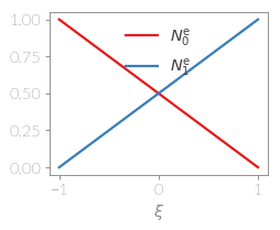
Linear Element
A one-dimensional linear element is defined using the nodes
| 0: | \(\xi = -1\) |
|---|---|
| 1: | \(\xi = 1\) |
where
Two-Dimensional Elements
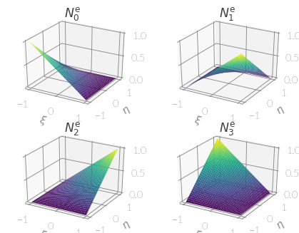
Linear Element
A two-dimensional linear element is defined using the nodes
| 0: | \(\xi = -1\), \(\eta = -1\) |
|---|---|
| 1: | \(\xi = 1\), \(\eta = -1\) |
| 2: | \(\xi = 1\), \(\eta = 1\) |
| 3: | \(\xi = -1\), \(\eta = 1\) |
where
-
Element.shape_function(xi, eta)¶ Return the shape function matrix of the element at the reference space position (xi, eta).
Parameters: Returns: The shape function matrix of the element at position (xi, eta).
Return type: